Analyse Guide
The Analyse module scores every heavy atom in the model against the debiased SNR map using MUSE (Model Uncertainty Score Estimator). MUSE adapts the EDIA methodology to any scalar field.
In screening mode (multiple experiments in one directory) the module also generates an interactive HTML summary report — the Screen Report — covering all crystals in a single sortable table.
Quick start
# Single experiment
pseudo-analyse --input_path /scratch/results/my_experiment

# Screening run (all crystals in the directory)
pseudo-analyse --input_path /scratch/results/my_screen --num_processes 8
CLI options
| Flag | Short | Default | Description |
|---|---|---|---|
--input_path |
-p |
required | Workspace root or single experiment directory. |
--stem |
-s |
auto | Explicit experiment stem. |
--map_path |
-m |
auto | Custom CCP4 map instead of the auto-discovered SNR map. |
--model_path |
auto | Custom PDB/CIF instead of the processed model. | |
--k_factor |
-k |
1.0 |
K factor used to locate the SNR map in quantify_results/. |
--map_cap |
-c |
50 |
Map cap used to locate the SNR map. Pass 0 for auto-detect. |
--num_processes |
-n |
1 |
Parallel workers for screening mode. |
--significance_alpha |
-a |
0.05 |
Significance level α for the null-distribution threshold. |
Python API
from analyse.api import run_analysis

run_analysis(
    input_path="/scratch/results/my_experiment",
    significance_alpha=0.05,
    num_processes=4,     # parallel for screening
)
Using MUSE directly
from analyse.muse.pipeline import run_muse, export_residue_csv, export_summary

result = run_muse(
    map_path="target_snr.ccp4",
    structure_path="target_updated.pdb",
    resolution=2.0,
)

print(export_summary(result))
export_residue_csv(result, "residues.csv")
Outputs
Per-experiment files
Written to <crystal>/analyse_results/:
| File | Description |
|---|---|
{stem}_atoms.csv |
Per-atom MUSE score, score_positive, score_negative, diagnostic flags |
{stem}_residues.csv |
Per-residue MUSEm, min/median/max atom score, diagnostic counts |
{stem}_summary.json |
Global statistics: OPIA, atom/residue counts, thresholds |
{stem}_scored.pdb |
Original structure with MUSE scores in the B-factor column (×100) |
Screening mode files
When multiple experiments are found the following are written to the screening root:
| File | Description |
|---|---|
index.html |
Interactive HTML screen report (see below) |
metadata/{stem}_screen_result.json |
Full per-experiment result dictionary |
metadata/screen_summary_{timestamp}.json |
Run-level summary: experiment list, mean OPIA, counts |
coot/{stem}_coot_view.py |
Auto-generated Coot session script per crystal |
Screen Report
The screen report is an interactive, self-contained HTML file written to <screening_dir>/index.html.
It aggregates every crystal’s MUSE results into one sortable table and provides direct links and Coot integration.
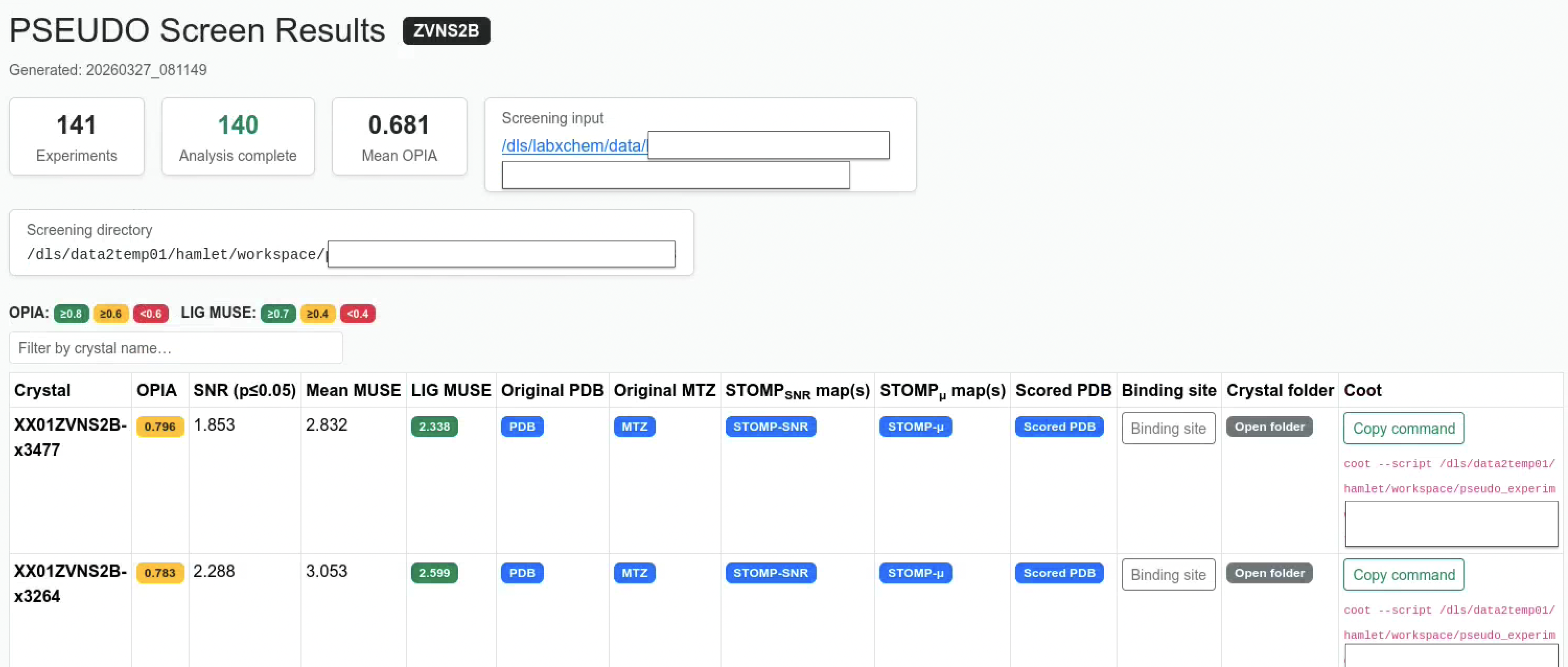
Summary cards
The top of the page shows run-level summary cards:
| Card | Description |
|---|---|
| Experiments | Total number of crystals discovered |
| Analysis complete | Crystals for which analyse_results/ exist |
| Mean OPIA | Average OPIA across all completed crystals |
| Screening input | Inferred original screening project directory |
| Screening directory | Path to the PSEUDO workspace root |
Table columns
| Column | Description |
|---|---|
| Crystal | Experiment stem (crystal name) |
| OPIA | Overall Per-instance Agreement: fraction of atoms with sufficient density support |
| SNR (p≤0.05) | The STOMP-SNR value at significance level p = 0.05, derived from the fitted null distribution |
| Mean MUSE | Mean per-atom MUSE score across the whole structure |
| LIG MUSE | MUSEm score for the ligand residue (default LIG) |
| Original PDB | Link to the input structure file |
| Original MTZ | Link to the input reflections file |
| STOMP_SNR map(s) | Link(s) to the STOMP SNR map(s) in quantify_results/ |
| STOMP_μ map(s) | Link(s) to the STOMP mean map(s) in quantify_results/ |
| Scored PDB | Link to {stem}_scored.pdb with MUSE scores in the B-factor column for PyMol visualization |
| Binding site | Toggle button revealing a table of all residues within 10 Å of the ligand |
| Crystal folder | Clickable link that opens the original crystal input directory in the file manager |
| Coot | “Copy command” button and selectable coot --script … command for Coot session loading |
Coot integration
Each crystal has a pre-generated Coot session script at coot/{stem}_coot_view.py.
Clicking Copy command copies the full coot --script <path> command to the clipboard.
Running the script in Coot loads:
| Map | Colour | Level |
|---|---|---|
| Original MTZ reflections | Brick red (0.80, 0.25, 0.10) |
σ = 1.0 |
| STOMP_μ (mean map) | Forest green (0.14, 0.55, 0.13) |
σ = 1.0 |
| STOMP_SNR map | Golden (0.85, 0.65, 0.13) |
Absolute STOMP SNR (p≤0.05) threshold |
# Make sure that coot is in your PATH
coot --version

# Or load coot.
module load coot

# For Diamond users coot is part of the ccp4 module:
module load ccp4

# Run from a terminal for visualisation
coot --script /path/to/coot/XX01ZVNS2B-x0051_coot_view.py
Regenerating the report
The report can be regenerated at any time without re-running analysis using the standalone command:
pseudo-screen-report --input_path /scratch/results/my_screen
pseudo-screen-report --input_path /scratch/results/my_screen --open_browser
--open_browser opens index.html in the default browser immediately after generation
Python API
from analyse.screen_report import generate_screen_report

generate_screen_report(
    screening_dir="/scratch/results/my_screen",
    lig_resname="LIG",          # residue name to score and centre Coot on
    neighbourhood_radius=10.0,  # Å radius for binding-site table
    open_browser=False,
)
Visualisation
Load {stem}_scored.pdb in PyMOL and colour by B-factor:
# PyMOL
load target_scored.pdb
spectrum b, red_white_blue
Python plots
from analyse.visualization import extract_residue_scores, plot_residue_profile, plot_water_support

scores = extract_residue_scores(result, score_field="musem", chain_id="A")
fig = plot_residue_profile(scores, title="Chain A — MUSE profile")
fig.savefig("chain_a_profile.pdf")

fig2 = plot_water_support(result, threshold=0.5)
fig2.savefig("water_support.pdf")
Significance threshold
When null-distribution parameters are present in metadata/ (produced by pseudo-quantify), pseudo-analyse automatically sets the OPIA and missing-density thresholds to the SNR value at p = significance_alpha. This adapts the scoring to the actual noise floor of the experiment. The threshold is reported in the SNR (p≤0.05) column of the screen report and embedded in {stem}_summary.json as significance_snr_threshold.
MUSE configuration
from analyse.muse.config import MUSEConfig, AggregationConfig, MapNormalizationConfig
from analyse.muse.pipeline import run_muse

config = MUSEConfig(
    map_normalization=MapNormalizationConfig(normalize=True),   # for 2Fo-Fc maps
    aggregation=AggregationConfig(opia_threshold=0.7),
)
result = run_muse("map.ccp4", "model.pdb", resolution=1.8, config=config)
See Configuration Reference — MUSE for all parameters.
HPC / SLURM submission
For fragment screening workspaces, wrap the command in sbatch and use --num_processes to parallelise across crystals within the job:
sbatch --partition cs05r \
       --cpus-per-task 8 \
       --mem-per-cpu 5G \
       --time 3-00:00:00 \
       --wrap "pseudo-analyse --input_path /scratch/results/my_screen \
                              --num_processes 8"
--num_processes controls how many crystals are processed in parallel inside the job. Set it to match --cpus-per-task.
References
- Meyder et al. (2017) J. Chem. Inf. Model. 57, 2437–2447.
- Nittinger et al. (2015) J. Chem. Inf. Model. 55, 771–783.